
Take a hypothetical watchlist of 400 liquid growth stocks and one fixed screen run after each Friday close. In the first week, 24 stocks clear a previously identified base pivot on volume at least 40% above their 50-day average. Seven weeks later the same screen, on the same 400 names, returns 8. Scan count breadth is the habit of tracking that number on purpose. Over those seven weeks the index in this example climbed 9.2% to a new high. The headline says the market is fine. The screen says the kind of setup the method trades has become a lot harder to find, and it can only say that because its definition stayed fixed long enough for the change to mean something.
Most breadth measures ask how many stocks are taking part in a move. A scan count asks something narrower: is the supply of opportunities that fit one specific breakout method growing or shrinking across the list you monitor? The two questions overlap, and they can still give different answers in the same week.
Four numbers that scan count breadth keeps apart
The term gets muddled because four different populations are often reported as one. Keeping them separate is most of the work.
- The eligible universe: every stock the screen is allowed to consider. In the example, 400 names with a price above $10 and average daily dollar volume above $20 million, with membership reviewed once a quarter.
- Stocks meeting setup conditions: names sitting in a base with a pivot already marked, close enough to trigger but still below it.
- Newly triggered breakouts: names that closed above their pivot during the observation window with the required volume. This is the count the example tracks.
- Breakout outcomes: what those triggered names did afterwards. That number can only be known weeks later.
A count of setups waiting to trigger and a count of breakouts that already triggered can move in opposite directions. A market that’s building many orderly bases can show a high setup count and a low trigger count at the same time. Neither one says anything yet about outcomes.
What has to stay fixed for the count to be comparable
A count from one week can be compared with a count from another only when four parts of the definition are identical: the universe, the pivot convention, the volume comparison and the observation time.
In the example, the pivot is the highest high of the base or its handle, marked before the observation week begins, so the screen can’t move the pivot to fit a breakout after the fact. The volume test compares breakout-day volume with the stock’s own 50-day average and requires at least 1.4 times that average. The observation time is the Friday close, using daily bars for the five sessions of that week. Change any one of those and the series gets a seam in it. Switching the volume test from a 50-day to a 20-day average, for example, changes which names pass in a way that has nothing to do with the market. A count that rises the week a filter was loosened is reporting the edit.
Writing the definition down in one line, and dating every change to it, is a cheap safeguard. The lesson on volume confirmation on breakout candles covers why the volume threshold matters for a single stock. For the count, the point is simpler: whichever threshold is chosen has to stay put.
Raw count versus share of the universe
The table below shows the three comparisons this lesson turns on. All figures are hypothetical.
| Observation | Qualifying breakouts | Eligible universe | Share of universe |
|---|---|---|---|
| Week 1 | 24 | 400 | 6.0% |
| Week 8 | 8 | 400 | 2.0% |
| Same 24, larger universe | 24 | 800 | 3.0% |
From week 1 to week 8 the count fell by 66.7% while the universe stayed the same, so the raw count and the share tell the same story. The third row is the trap. Suppose the universe is widened to 800 names and the screen again returns 24. The raw count looks unchanged, yet the share has halved to 3.0%. To match the original 6.0% on the larger list, 48 names would need to qualify.
Reporting the share alongside the count, with the denominator written next to it, prevents a quiet universe change from reading as stable conditions. If the universe changes, the old series and the new one are best treated as two different series.
One stock, several scans, one opportunity
Breakout traders rarely run a single screen. A typical set might include the pivot breakout scan, a 52-week-high scan and a pocket-pivot scan. In a hypothetical week those return 24, 31 and 15 names, a total of 70 hits. Once duplicates are removed, there are 46 different stocks, and 7 of them appear on all three lists.
Adding the three counts together overstates the supply of distinct opportunities by 24 names. A stock that shows up on three screens is one stock with three descriptions. It may deserve closer attention for that reason, but it carries one set of earnings dates, one set of holders and one chart. Counting it three times treats correlated evidence as independent evidence.
The same applies across time. Of the 24 names on this week’s pivot scan, 9 were also on last week’s list and 15 are new. A list that’s mostly repeat names describes a few stocks holding their breakout zone; a list that’s mostly new names describes fresh supply. Tracking the new-name count as its own column keeps those two situations apart.
Reading the count next to the index
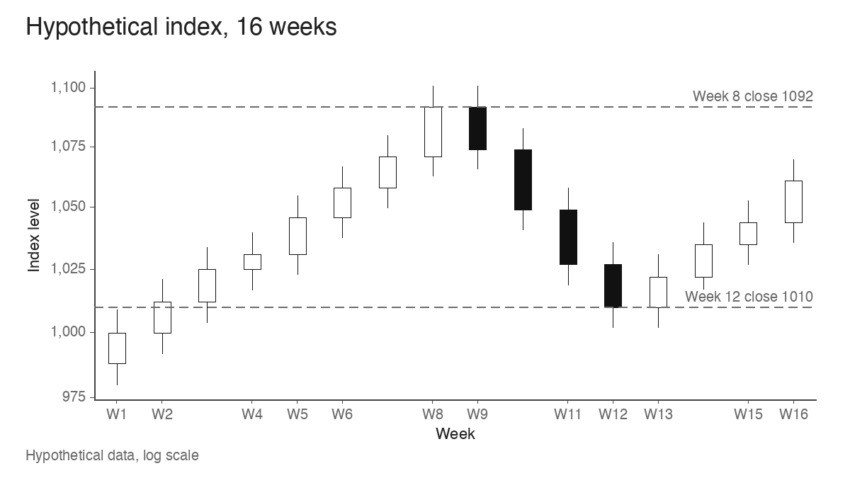
The hypothetical index below runs for 16 weeks. From week 1 to week 8 it rises 9.2%, closing at 1092 after a weekly high of 1101. It then falls 7.5% to a week-12 close of 1010 and starts rebuilding, reaching 1061 in week 16, still 2.8% below the week-8 close.
The weekly pivot-scan count from the same hypothetical universe of 400 tells a different story. It falls steadily from 24 to 8 while the index climbs to its high, bottoms at 3 in weeks 11 and 12, and then recovers to 19 by week 16, while the index is still under its prior high.
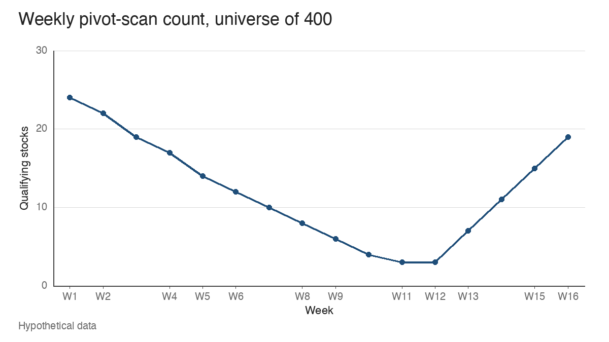
Two readings follow, and both are observations that need context. In weeks 1 to 8, a rising index with a shrinking count suggests the advance is being carried by fewer names that still fit the method; the stocks that broke out earlier may be extended, and fewer new bases are resolving. In weeks 13 to 16, a count climbing from 7 to 19 while the index is 2.8% below its high suggests that individual stocks are setting up and triggering before the average confirms anything.
Neither pattern switches exposure on or off by itself. A trader using this measure might look for agreement from the other tools that describe the same tape: whether the index has logged a follow-through day after a correction, whether the advance-decline line is confirming or diverging, and whether the new highs and new lows lists are expanding on the right side. A rising scan count with a falling advance-decline line is a narrower recovery than one where both improve.
Supply of setups versus whether they’re working
A count describes how many opportunities the method is finding. Whether those opportunities are paying is a second question, and it needs a follow-up on the same names.
Take the 24 week-1 breakouts and check them four weeks later. In this hypothetical cohort, 10 are still holding above their pivots (41.7%), 8 have slipped back inside their bases (33.3%) and 6 have fallen far enough to trigger a typical stop below the pivot (25.0%). A high count followed by a cohort where most names lose their pivots is a different market from a high count followed by most names holding. The failed breakout lesson covers how a single name gives that signal; the cohort view simply counts how often it’s happening across the list.
The count and the follow-up answer separate questions, so they’re best kept as separate columns: how many triggered this week, and what share of a cohort from four weeks ago is still above its pivot. A burst of 24 qualifying breakouts can still fail as a group, and the follow-up column is what shows that.
Where the count misleads
Several practical problems can make a scan count say more, or less, than the market is offering.
A restrictive filter suppresses the count. If the screen also requires every name to pass the full trend template and a minimum relative strength rank, a reading of 3 may reflect the strictness of the filter as much as the scarcity of setups. That’s acceptable when the filter is the method, but it means a low reading in a strict screen and a low reading in a loose one aren’t comparable.
One industry can dominate. If 11 of the 24 week-1 names are semiconductor stocks, that group supplies 45.8% of the list. Strip them out and 13 names remain, 3.25% of the universe. The headline count would look healthy even if one group were carrying the method. A quick industry column on the scan output shows when that’s happening.
Data changes distort comparisons. Split adjustments, a vendor revising volume history, an index reconstitution feeding the universe, or a holiday-shortened week with four sessions can all move the count without any change in the stocks. Noting these events on the series, week by week, is the practical way to know which jumps to discount.
Finally, a count is a sample. A custom scan describes one method applied to one universe at one observation time. It can’t establish the condition of every stock in the market, and it can’t predict the next index move. The William O’Neil approach to leading stocks reads individual leaders alongside the general market, and a scan count fits that same supporting role.
Keeping one definition long enough to learn from it
The value of a scan count comes almost entirely from consistency. A written definition, a fixed universe with its size reported, a de-duplicated list with new names flagged, and a cohort follow-up turn a noisy screen output into a series that can be read week to week. In the example, the drop from 24 to 8 against a rising index and the recovery from 3 to 19 before the index regained its high were both visible only because none of those parts changed in between.
Learn the pattern. Ride the trend. Keep the gains.
Educational content only. Not investment advice. Trading involves risk. You are responsible for your decisions.
Get the free Market Wisdom e-book
Join Trends and Breakouts — historical winners, breakout studies, and risk lessons. No spam, unsubscribe anytime.